Modal logic

Background

In the last few decades, there has been a huge push to use phonetic distributions to argue about underlying (phonological) categories. Researchers have even argued that children pay attention to distributional evidence for categories (Kuhl 2000). One way in which distributional evidence has been used is by looking at peaks or modes in the distributions to learn about underlying categories.

Today’s blog post is about the issues that arise with mode detection. I will make two main points. First, that using observed distributions and observed modes to study underlying categories is really fraught, largely due to sampling variation/error. Second, even if we solve such worries with larger sample size or multiple replications of a study, there is still the issue that the abstract mixture distribution that is the result of two or more categories itself will not have more than one mode below a certain threshold. Consequently, once we are below that threshold, there is simply no way to tell how many categories are there underlyingly, and any bi- or multi-modality we see in the observed distribution is simply noise.

OK, I have been throwing around some terms above, so it is best to be clear about some of them. When it comes to mixture distributions, it is important to clearly distinguish between three important concepts.

1. Observed distribution
1. Underlying distributions
1. Mixture distribution

An observed distribution is the distribution based on our data. The underlying distributions are the abstract distributions of the (causal) categories we are interested in. The mixture distribution is the abstract distribution that we get when there are two or more categories that are mixed to give us a distribution.

Throughout, I will simulate an infinite population with a size of 10,000,000 to make the modelling easier to follow and to focus on the main point. For the sample size of a single experiment, I will use 100.

What can we learn from the observed distributions?

Very often researchers look for peaks or modes in the distributions to infer the number of underlying categories. However, this is complicated by randomness (damn you, randomness!!). I have talked about randomness rearing its ugly head in previous blogposts too in the context of individual variation Durvasula (2025b) and near mergers (Durvasula 2025a).

An observed distribution can be bimodal (or multimodal) through sampling error even if there is a single underlying distribution; and an observed distribution can be unimodal even if there are two or more underlying distributions due to sampling error. In the simulation below, I replicated cases where there is a single underlying distribution and those where there are two underlying distributions.

First, we need to model two underlying category distributions as normal distributions. As can be seen from the plot and the code, the two underlying categories differ only in the means of the distributions.

hide

library(tidyverse)
library(gridExtra)

# Setting plot theme
theme_set(theme_bw())

# Defining the underlying distributions
set.seed(100)
sd=20
Underlying1 = rnorm(1e7, mean=100,sd=sd)
Underlying2 = rnorm(1e7, mean=120,sd=sd)

plot1 = data.frame(Underlying1) %>% ggplot(aes(Underlying1)) + geom_density()
plot2 = data.frame(Underlying2) %>% ggplot(aes(Underlying2)) + geom_density()
grid.arrange(plot1,plot2,ncol=2)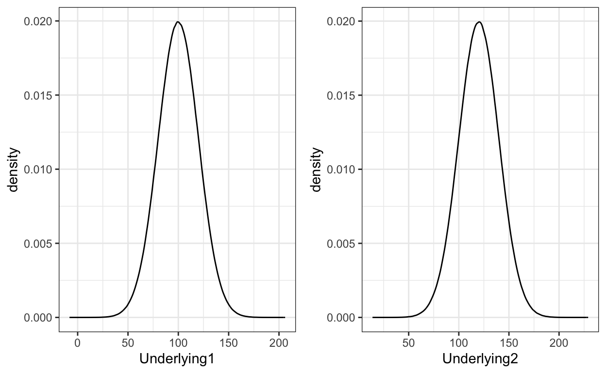

Next, we need to create the abstract mixture distributions, wherein the first mixture distribution actually consists of just a single underlying category (so this is a degenerate mixture distribution), and the second one consists of two underlying categories. Then finally, let’s get three samples from each of the abstract mixture distributions. As can be see from the plots, one can see bimodality in some of the simulations when there is only a single underlying category (top row of the figure), and one can see unimodality in some of the simulations even when there are two underlying categories.

hide

# Defining the mixture populations
# Single underlying distribution
Mixture1 = Underlying1
# Two underlying distributions
Mixture2 = c(Underlying1,Underlying2)

# Sampling from the mixture distributions
sampleSize=100
NumSamples=3
set.seed(10)
Simulation1=data.frame(expand.grid(1:NumSamples,c("Dist1","Dist2"))) %>% 
  rename(Sample=Var1,Distribution=Var2) %>% 
  slice(rep(1:n(), each = sampleSize)) %>% 
  mutate(Simulations = ifelse(Distribution=="Dist1",sample(Mixture1,sampleSize*NumSamples,replace=T),
                              sample(Mixture2,sampleSize*NumSamples,replace=T)))

# Plotting
Simulation1 %>% 
  ggplot(aes(x=Simulations))+
  geom_density()+
  facet_grid(Distribution~Sample,scale="free")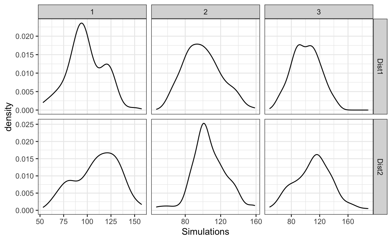

Figure 1: Simulated samples from a distribution that consists of a single (top row) and two (bottom) underlying categories.

So, for a single experiment, one can’t look at the observed distribution and tell whether there are one or two or many underlying categories — that would simply be an exploration in noise.

One could imagine trying to solve the problem with increased sample size. But, there is no sample size where we can be sure that we have a clear reflection of the actual mixture distribution — all we know is that as the sample size increases, it will tend to the abstract mixture distribution, but this is very different from saying anything specific about any particular sample size. So, really, that leaves us with replications. As Ronald Fisher put it in the context of inferring from p-values, replications are king.

``we may say that a phenomenon is experimentally demonstrable when we know how to conduct an experiment which will rarely fail to give us a statistically significant result.’’ (Fisher 1935, 16)

So, perhaps, one can solve the problem by repeating the experiment many times and seeing if in general you get one or two or many modes. A more general lesson here is to not fall prey to the temptation of trying to interpret the results of a single experiment. Relatedly, p-values have a uniform distribution under the null hypothesis (Soch 2024); therefore, an isolated case of a low p-value in an experiment is not evidence for anything, since you could have gotten any p-value by random chance. But the same reason applies to all statistics — you are always at the mercy of Mr. Random Variation.

As always: But wait, there’s more!

Of course, the problem gets worse!¹ One might be tempted to think that this is just all science — of course, we should replicate; of course, no single experiment should count by itself; and when we phrase things a certain way in our papers, that is just rhetorical, no one really falls prey to it. Don’t be stupid, Karthik!

First of all, I have heard too many folks cite some odd paper with some data as crucial to make a point. So, yes, I am naive, but I ain’t alone!

Second, the big problem is that under some conditions, no sample size or replication is going to help you identify the underlying categories. Even the abstract mixture distribution of two or more underlying distributions can be unimodal under some circumstances (Sitek 2016; Murphy 1964). If the underlying distributions have:

(a) close means
(b) or large variances
(c) or imbalanced sizes

So, forget the sampling error issue, mathematically, we know that for any mixture of normals, there is a sufficient threshold below which one expects the abstract mixture distribution to be unimodal, even if there were two underlying category distributions.

\[\begin{equation} |Mean_1 - Mean_2| ≤ 2*min(σ_1, σ_2) \end{equation}\]

So, no mode test can be successful at identifying the underlying distributions (one vs.~two vs.~many) below that threshold.

You can see the abstract mixture distributions below where I vary the mean of the second category. Note, these distributions represent the populations, not samples, as they use huge sizes.² As can be seen in the plot below, the abstract mixture distribution shows bimodality only when the means are sufficiently far apart. Visually, this appears when Mean2=150, when the difference in the means is 50. Note, this is more than twice the standard deviation (20), as expected as per the inequality above.

hide

mean1=100
mean2=c(110,120,130,140,150)

expand.grid(mean1,mean2) %>% 
  rename(Mean1=Var1,Mean2=Var2) %>% 
  slice(rep(1:n(), each = 2e7)) %>% 
  group_by(Mean2) %>% 
  mutate(Simulations = c(rnorm(1e7,mean=Mean1,sd=20),rnorm(1e7,mean=Mean2,sd=sd))) %>% 
  ggplot(aes(x=Simulations))+
  geom_density()+
  facet_grid(~Mean2)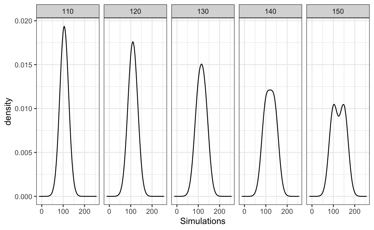

Mode tests

To summarise, observed distributions are really bad at telling us about underlying categories. But, the real problem is that below a threshold, the abstract mixture distribution itself is not going to have more than one mode. So, if you try to run some sort of mode test (say Hartigans’ Dip) on the observed distributions, below a certain threshold, it is useless – and no statistical jiggery-pokery will help you. And in fact, if a statistical test (say, AIC, BIC, null hypothesis test) does give you a result below that threshold, it is simply the bias of the test, not a believable result.

Below I show simple simulations for different underlying populations or distributions. I keep distribution₁ the same in all the cases, but vary distribution₂ in terms of means above and below that of distribution₁. I also mark the region within which, mathematically, one expects a single mode, with vertical dashed lines. I conducted the simulation for two different sample sizes (N = 1000/distribution, and 100,000/distribution), and get a Hartigans’ Dip statistic for each simulation — these values are plotted in the figure.

As can be seen, Hartigans’ dip scores are the same for the mean differences within the mathematical limits for unimodality. This is true for both smaller and larger sample sizes.

What’s worse, the null hypothesis for the Hartigans’ test (and many other such tests) is that there is a single underlying category distribution, and the lack of a statistical significance is often interpreted as evidence of absence of two or more categories — that is evidence of a single category. But, we know that mode tests cannot identify the true underlying modes below a threshold, so it is a bit like saying there is no difference between the weight of a hydrogen atom and a uranium atom because a bathroom scale can’t tell them apart.

hide

    # Hartigan's dip test
    library(diptest)
    library(tidyverse)

    mean_1=0
    sd_1=1
    sd_2=2

    # Getting a function
    HDSimulation=function(size=1e5,mean1=mean_1,mean2=2,sd1=sd_1,sd2=sd_2){
      # Creating the first distribution
      dist1 = rnorm(size,mean=mean1,sd=sd_1)
  
      # Creating the second distribution
      # And mixing it with the first
      dist2 = rnorm(size,mean=mean2,sd=sd2)
      totalDist = c(dist1,dist2)
  
      # Return the Hartigans' Dip statistic
      return(dip.test(totalDist, simulate.p.value = FALSE, B = 2000)$statistic)
    }
    HDSimulation=Vectorize(HDSimulation)

    # Simulating Hartigans' dip for different pairs of distributions
    Results=expand.grid(sampleSizes=c(1e3,1e5),mean2Range=seq(-10,10,by=1)) %>% 
      mutate(HDip = HDSimulation(size=sampleSizes,mean2=mean2Range))

    # Plotting the results
    Results %>% 
      ggplot(aes(mean2Range,HDip))+
      geom_line()+
      xlab("Mean2 value")+
      facet_grid(sampleSizes~.)+
      theme_bw()+
      # Adding threshold for unimodality
      geom_vline(xintercept=2*min(2,1),linetype="dashed")+
      geom_vline(xintercept=-2*min(2,1),linetype="dashed") +
      annotate(geom="text",x=0,y=0.075,label="region of \n unimodality")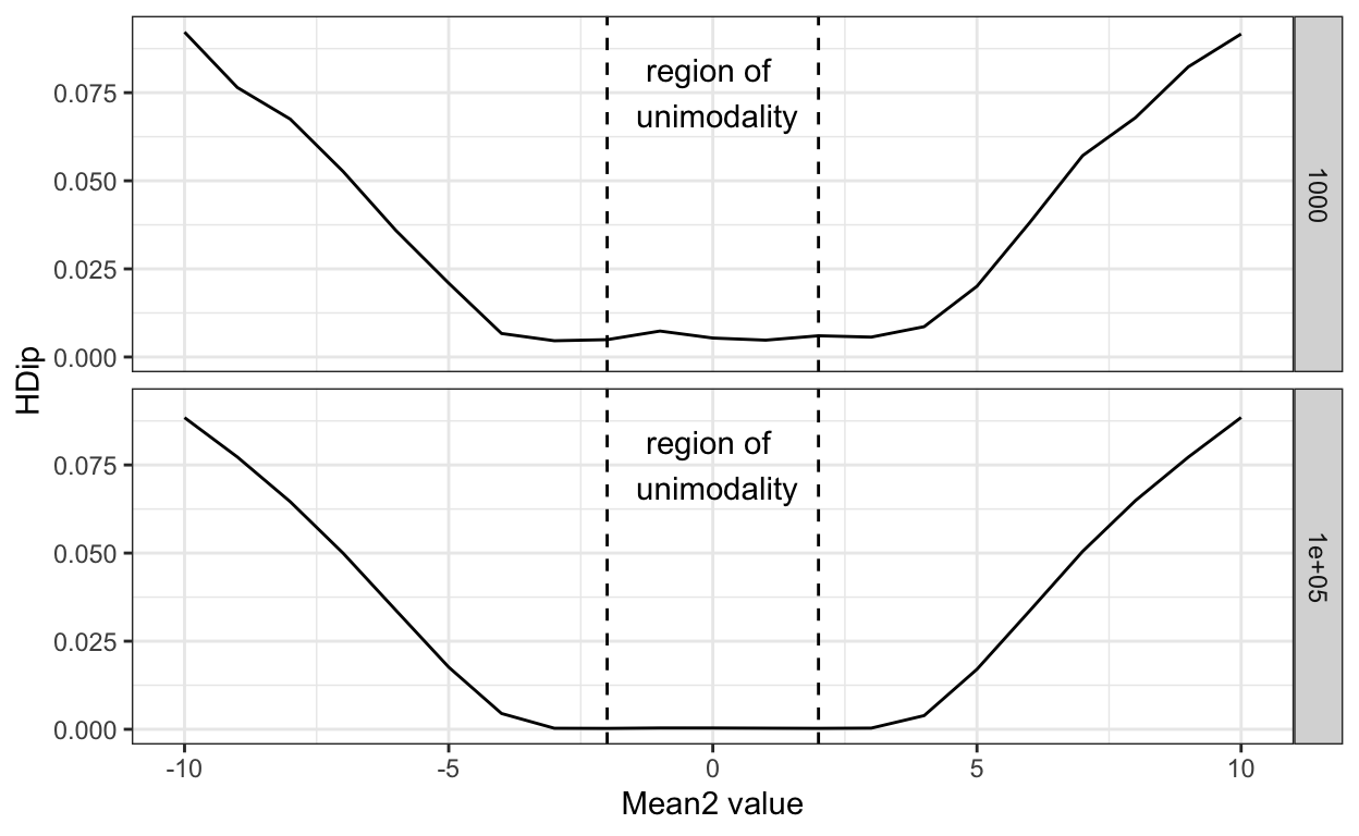

The truth is that below a threshold, such tests are useless, and even above the threshold, we don’t know if we are succumbing to random variation or differences in underlying category structure for any single experiment.

Conclusion

Replication helps, when the mean differences are quite large (relative to the variances). But, when the underlying differences are quite large and replicable, we don’t need fancy statistics, the inter-ocular trauma test is good enough. We need help when the underlying differences are small — these are the more interesting case, but it is exactly in this case that the mode test fails.

Furthermore, as Murphy (1964) correctly put it ``It is one thing to argue from mechanisms to expected outcomes; it is very much more difficult and hazardous to argue from observations back to mechanisms.’’ (p. 312).

Instead of looking at data and trying to tea-leaf read, we need precise enough theories that make precise predictions about the mixture distribution(s) that we can go test. Now, even that is not going to sovle all our problems, but it is at least approaching the problem the right way. Sadly, in Phonetics, we are really far away from this first step. At this current stage of our understanding, the best bet for categoryhood we have is phonological patterning/activity, as I have discussed in previous blog posts (Durvasula 2025a, 2024).

A student of mine, Huanbin Teng, is looking at the more general issue of category overlap and common statistical tests. Stay tuned for his paper soon, that will include formal results, simulations, and finally testing of different statistical techniques.

---

1. That’s how I write all my blog posts, apparently!↩︎

2. OK, they are still samples, but really HUGE ones! Again, this was done to make the code easy to follow.↩︎